
Introduction To Deep Q-Learning
Recently, I was fortunate enough to be awarded the Data61 summer research scholarship from the CSIRO. This is the first of a 2 part series detailing what I learned, the conclusions I came to and some mistakes I made along the way. My chosen topic was Machine Learning For Self-Driving Cars. This installment outlines Deep Q-Learning with a basic, high level example. The next walks through an implementation that learns to control a simulated car driving on a simulated stretch of highway. The end goal of the project is to sufficiently train a model to control an RC Car, then maybe something larger if all goes well.
Inspired by recent developments in self-driving car technology; an eagerness to experiment with machine learning and the work done by Deep Mind, I decided to jump in the deep end and try to implement a Deep Q-Network. I later realized that it was a bit ambitious for my first taste of neural networks to be a CNN implementing Deep Q-Learning. However, here we are. If you don’t push yourself, you’ll never improve…right?
Table Based Q-Learning
Lets start from the beginning. Table based Q-Learning (note: Not Deep Q-Learning) is a type of reinforcement machine learning. Q-Learning was first detailed in a Cambridge PhD thesis by Christopher Watkins in 1989. It is inspired by how you would normally train an animal or child. You REWARD desirable behavior and punish (negative REWARD) undesirable behavior.
Now for some terminology.
An AGENT has a STATE. The STATE consists of the observations the AGENT can make. The AGENT can select an ACTION that will then transition it to another STATE. Each ACTION is ranked by the potential it will result in a REWARD, this is known as the action’s QUALITY.
For an example almost everywhere I have looked goes through the Hello World of Reinforcement Learning, ‘Grid World’. For a change of scenery I’ve adapted a tongue in cheek example from my many years of bar-tending.
Consider the image and table below. The person (agent) is in a bar, and can occupy one of the below states;
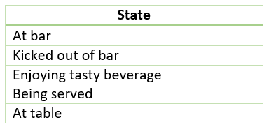
The agent can occupy one of these discrete states
From each state the agent can select from of the below actions.
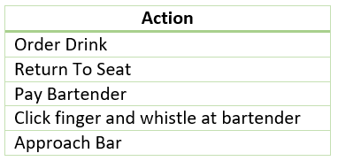
The agent can select one of these discrete actions
Finally each action is associated with a quality, for now we’ll initialize them all as zero, but note,* after training, the quality of an action varies between states. Also, *‘Terminal’ indicates a state that ends the simulation.
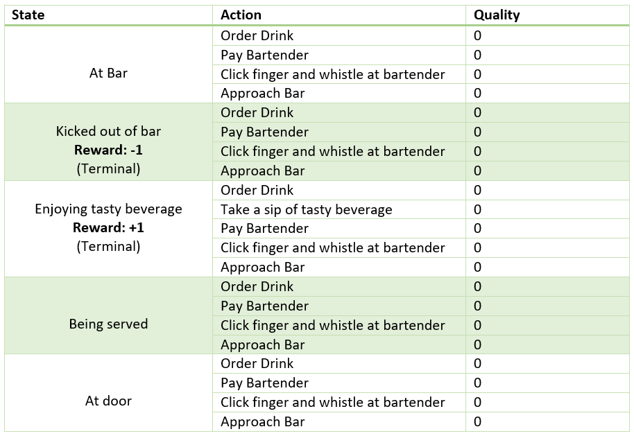
The full Q-Table. In each state the agent can select on action. The 'quality' will be updated depending on the reward. At test time the agent just selects the action with the highest reward.
Rewards are not necessarily ONLY associated with terminal states. That’s just how this example works.
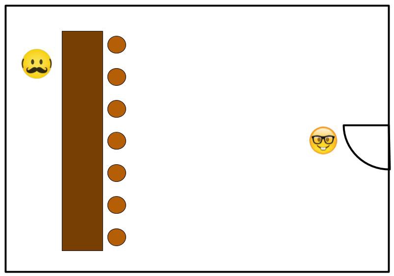
A nerd walks into a bar ...
From the current state *(At door) it is easy for us to see the best *action would be, ‘Approach bar’. Followed by, ‘Order drink’, ‘Pay bartender’, then ‘Take a sip of tasty beverage’. (Note: ‘Click finger and whistle at bartender.’ is NEVER a good action). The goal of Q-Learning is to determine the correct action to take given the current state, this is known as the policy.
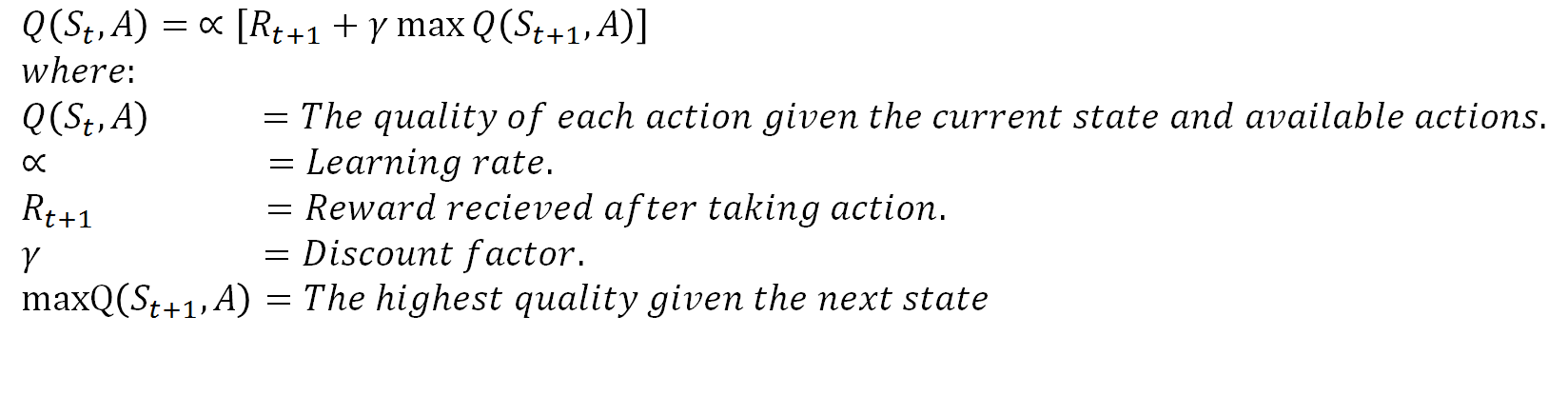
Q-Learning does this via the use of the *Bellman *equation:
---
A few things to note;
- learning rate is a value from 0 → 1 that controls how much the algorithm overwrites the current $Q-value$ with newer information.
- discount factor is also a value from 0 → 1 that controls how much you trust the future $Q-value$ prediction
- if, after an action the agent finds itself in a terminal state the equations is simply:

---
So, initially the agent takes random actions. These actions result in a change in state and a potential reward (either positive or negative). The reward resulting from the state-action pair is then updated in the Q-Table. By continually selecting the action with the highest quality the algorithm converges of a policy that maximizes the rewards received.
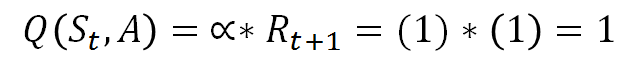
Imagine after a bunch of random actions the agent finds itself in the ‘being served’ state. Randomly the agent selects the action *‘Pay bartender’, *resulting in a new state *‘Enjoying tasty beverage’ *and a reward of +1.
Applying Bellman’s equation for a terminal state, the quality *of the *state-action pair is updated (setting *alpha *to 1 for simplicity) we arrive at:
Bellman Equation
which we then update in the Q-table

---
Now, the next time the agent finds itself in the ‘being served’ state it will know to take the action ‘Pay Bartender’. What’s really cool is that next time the agent finds itself in the ‘At Bar’ state, Bellman’s equation will look like this (assuming gamma = 1)
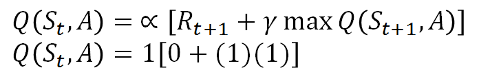
---
So the quality of the state-action pair ‘At Bar — Order Drink’ *gets updated. This process of working backwards from goal state start state continues until eventually a clear path from ‘At Door’ to ‘Enjoying tasty beverage’* is defined.
So all together the algorithm looks like this:
setup q_table
initialize state, alpha, gamma

while training:
  get q values for each action given the state
  select action with highest q
  apply action
  observe reward
  observe next_state
  if next_state is terminal:
    q_update = reward
  else:
    get q_next values for each action given the next_state
    observe the largest q value (q_max) in q_next
    q_update = alpha*(reward + gamma*q_max))

  q_table[state][action] = q_update
  state = next_state
So that’s Q-Learning, we can all go home now…not quite. There are a few bumps in the road some of you may have spotted.
Exploration vs Exploitation
Some of you may have noticed that once the agent discovers a state-action pair that results in a reward it has no incentive to explore other possibilities. It’s kind of like selecting the first cocktail on the menu every-single-time. Algorithmically it makes sense, assuming the cocktail was crafted by a skillful bartender and served with a smile. You experienced the reward of a tasty beverage from selecting the first cocktail on the list, why would you explore further than that? When just 2 places down is the Last Word cocktail…clearly the optimal choice!
The is the exploration vs exploitation problem. Fortunately there is something we can do about it known as the Epsilon Greedy *implementation of Q-Learning. In *epsilon greedy each iteration, with a probability of epsilon, the agent takes a random action as opposed to action with the highest quality. This forces the agent to explore more of the state space early in training. As training progresses we slowly reduce epsilon to some predefined minimum in order to favor exploitation over exploration.
setup q_table
initialize state, epsilon, alpha, epsilon, decay_rate

while training:
  get q values for each action given the state

if (epsilon > random_float_between_0_and_1):
    select random action
  else:
    select action with highest q

apply action
  observe next_state
  observe reward
  if next_state is terminal:
    q_update = reward
  else:
    get q_next values for each action given the next_state
    observe the largest q value (q_max) in q_next
    q_update = alpha*(reward + gamma*q_max))

  q_table[state][action] = q_update
  state = next_state
  epsilon -= decay_rate
The problem of efficiency
The next problem is in the rate at which out Q-Table grows with complexity. Even for our simple bar example we have 20 entries. Even for a simple tic-tac-toe game, accounting for symmetries and other reductions there are almost 27,000 possible game combinations (I didn’t work that out, if you’re interested you can click here). As you can imagine, for any application with any real complexity, the Q-Table is not going to cut it.
Enter Q-Net
This is what prompted the use of an artificial neural network to approximate the behavior of a Q-Table. In 2013 DeepMind released ‘Playing Atari With Deep Reinforcement Learning’ and 2015 ‘Human-Level Control Through Deep Reinforcement Learning’
To make this work we’re going to need to make a few modifications. First, because we use gradient decent to train neural networks and learning rate (alpha) is included in the gradient decent algorithm we can drop it from Bellman’s equation.
We can now use this equation as a target to calculate our loss function. For this we’ll take the Mean Squared Error *(MSE*) error between the Q-value predicted by the neural network and the result of the above modified Bellman’s equation.
To train an NN in place of a Q-Table we do two feed-forward passes and one back propagation pass. On a forward pass we use the state as the input. The output is 1xN matrix representing the quality value for each possible action.
The first we pass the state through the NN to get an estimate of the quality *for each *action. Then, just at when using the Q-Table we select the action *with the highest *quality *and apply that *action.
We then observe the next state, and pass it through the NN. We then observe the largest Q-Value in the output and use the modified Bellman equation to calculate a target value. Finally we calculate the mean squared error between the first forward pass and the target then back propagate it back through the NN.
Here it is in flowchart from:
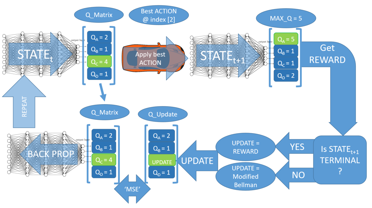
Flowchart of Deep Q-Learning training loop
Following is an epsilon greedy pseudo code implementation for training a Deep Q-NN:
initialize state, epsilon, alpha, epsilon

while training:
  observe state
  feed state forward through NN to get q_matrix
  if (epsilon > random_float_between_0_and_1):
    select random action**
  else:
    action_idx = index of the element of q_matrix with largest value

apply action at action
  observe next_state
  observe reward
  if next_state is terminal:
    q_update = reward
  else:
    feed forward next_state through NN to get q_matrix_next
    observe the largest q value (q_max) in q_matrix_next
    q_update = reward + gamma*q_max

  make copy of q_matrix (q_target)
  q_target[action_idx] = q_update
  loss = MSE(q_matrix, q_update)
  optimize NN using loss funciton**
  state = next_state
  epsilon -= decay_rate
Catastrophic Forgetting
We’re getting there, almost time for some real code. We have one final problem to solve before we put code to IDE (well there are plenty more additions we could add to this, but for now, this should get us by).
What is catastrophic forgetting, it sounds intimidating. This is a artifact of training a neural network with gradient decent. It occurs during training when the neural net receives, what it perceives as conflicting information.
For an example I’m going to leave the simple bar simulation behind and focus on the highway simulator we’ll be training in later. In the frame below the agent is the red car and the obstacles are the gray cars. The lines protruding from the red car represent the simulated LiDAR. The agent uses LiDAR data as it’s state. Each beam returns the distance to the object it hits. If a beam does not hit anything it will return a value equal to the range of the LiDAR. The red circle is for collision detection. Horizontal lines are lane markers that are purely aesthetic. A +1 reward is award each frame if the agent doesn’t collide with an obstacle. A -1 is awarded is there is a collision. The agent can ‘accelerate’, ‘break’, ‘veer left’, ‘veer right’ or ‘do nothing’. The ‘do nothing’ action just means the agent will continue on its current path at a constant velocity.
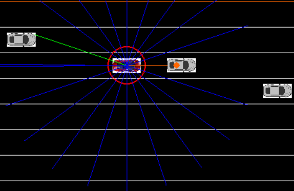
Agent (red), Obstacles (Gray)
Now back to catastrophic forgetting. While training, the Q-Net comes across the situation above. The agent gaining on a slower car in the same lane. Using the *epsilon greedy *implementation the agent selects *‘veer left’, *avoiding the car and receiving a +1 reward. This results in a low error which is back-propagated through the network, promoting this behavior in the future. So what’s the problem?
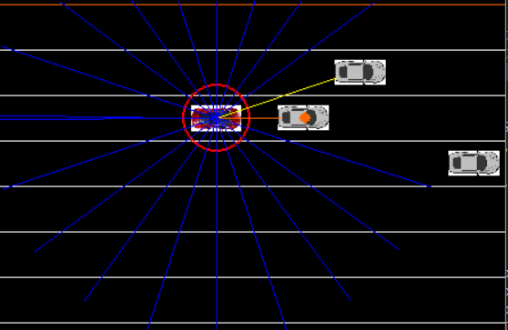
Now consider the situation below.
---
Here we also have a slow car in the same lane. To a young Q-Net the 2 states may look quite similar. The state is fed through the Q-Net resulting in ‘veer left’ but this time it results in a collision and a -1 reward. This results in a large error that is back propagated through the network erasing what we learned the jut before. Fortunately there is a solution.
Experience Replay
This is the final addition we need to have before we put it all together. If you’re familiar with supervised learning, experience replay is similar to batch optimization. The aim is to smooth out the training process by constantly updating a buffer of past experiences, then, each loop training on a randomly selected batch taken from the buffer.
Initially we will be filling the buffer with random samples, but how does data logged by randomly controlling the agent help at all? The idea is that by training on a batch the Q-Net will be less likely to be affected by catastrophic forgetting, additionally, as the Q-Net becomes better at correctly estimating the quality of an action the agent will make better decisions. These will in-turn overwrite the less relevant random data.
What is really cool, and something many of you may have already figured out. There is no reason we could not fill our buffer with data logged by a human controller. Therefor providing the Q-Net with meaningful data from the start. In fact, I will add this feature towards the end of the post.
